Normalizing Flows: Density Estimation by Change of Variables

Normalizing flows make a very explicit trade:

• If you can build an invertible map with a tractable Jacobian,
• then density estimation becomes straightforward: exact likelihoods via change-of-variables.

The architectural challenge is to make both the inverse and the Jacobian determinant cheap enough to evaluate. When that is possible, the model can optimize log-likelihood directly.

The equations below describe a continuous-density flow with an invertible differentiable map and a tractable Jacobian determinant. Dinh, Sohl-Dickstein and Bengio’s Real NVP paper gives the coupling construction and evaluated image-model experiments.

From a Base Distribution to a Data Density

The central idea is to model a complex data distribution by transforming a simple, well-defined base distribution (usually a standard multivariate Gaussian).

We define a deterministic and invertible function such that:

Because is invertible, we can also go backward: . Together with a tractable Jacobian determinant, this inverse lets us evaluate the model density. Exact evaluation does not mean that the model exactly matches the data distribution.

The Change of Variables Formula

To relate the density of our complex data to our simple latent space, we use the Change of Variables Formula. For a diffeomorphism between spaces of the same dimension, with , the relationship between densities is:

Here, is the Jacobian of the inverse transformation. The determinant of the Jacobian accounts for how the transformation stretches or compresses the "volume" of space. If the function pulls points apart, the density decreases; if it pushes them together, the density increases.

Training via Log-Likelihood

In practice, we don't maximize the likelihood directly because products of many density values can underflow or overflow. Instead, we use the Log-Likelihood:

In code, the training objective is usually implemented via the inverse pass (because you need anyway):

The expectation is over the training-data distribution, approximated by a minibatch average. Map each example to latent space, score it under the base density, and add the log-determinant correction.

Sign convention (the common confusion):

• At corresponding points , .
• Training via the inverse is convenient because is required to evaluate .

Why the Logarithm?

• Numerical Stability: It turns products into sums, preventing our computers from rounding small values to zero.
• Easier Optimization: The logarithm is monotonic. Maximizing the log-likelihood is mathematically equivalent to maximizing the likelihood itself.
• Additive Contributions: Each example and each Jacobian factor contributes a separate term to the objective.

Building Deep Flows: The Power of Composition

A single affine transformation cannot turn a Gaussian into a two-moons density. Composing nonlinear invertible layers provides a more expressive family while preserving invertibility.

If we have layers:

The log-determinant of the total Jacobian is the sum of the layer log-determinants, each evaluated at that layer’s input:

Thus tractable layerwise determinants remain tractable under composition.

Real NVP Coupling Layers

One of the most influential flow architectures is Real NVP (Real-valued Non-Volume Preserving). It uses Coupling Layers to ensure the Jacobian is easy to calculate while remaining highly expressive.

The Coupling Mechanism

First split the coordinates as . An affine coupling layer leaves one block unchanged and transforms the other:

1. Identity Part: .
2. Transformed Part: .

The networks and need not be invertible: the unchanged coordinates supply their inputs during inversion. Solving for the second block gives .

For the code below, use a binary mask and let . Networks then return -dimensional vectors, with outputs on masked coordinates ignored:

Alternating masks lets each coordinate be transformed across layers.

The Jacobian determinant:

Because doesn't depend on , and depends on only element-wise, the Jacobian is block lower triangular when coordinates are ordered as the two blocks. The determinant of a triangular matrix is just the product of its diagonal elements.

To compute the log-determinant, you never form the Jacobian. Sum the relevant entries of :

That’s why coupling layers scale: the log-det is an reduction, not an matrix determinant.

A Minimal Coupling Layer in PyTorch

This layer implements the forward map, inverse, and their log-determinants for batches of vectors. It is a building block rather than a complete training experiment.

import torch
import torch.nn as nn

class CouplingLayer(nn.Module):
    def __init__(self, data_dim, hidden_dim, mask):
        super().__init__()
        self.register_buffer("mask", mask.detach().clone().float())
        # Neural networks for scale and bias
        self.s_net = nn.Sequential(nn.Linear(data_dim, hidden_dim), nn.ReLU(), 
                                   nn.Linear(hidden_dim, data_dim))
        self.b_net = nn.Sequential(nn.Linear(data_dim, hidden_dim), nn.ReLU(), 
                                   nn.Linear(hidden_dim, data_dim))

    def forward(self, z):
        z_a = z * self.mask
        s = torch.tanh(self.s_net(z_a))
        b = self.b_net(z_a)
        x = z_a + (1 - self.mask) * (z * torch.exp(s) + b)
        log_det_J = ((1 - self.mask) * s).sum(dim=1)
        return x, log_det_J

    def inverse(self, x):
        x_a = x * self.mask
        s = torch.tanh(self.s_net(x_a))
        b = self.b_net(x_a)
        z = x_a + (1 - self.mask) * ((x - b) * torch.exp(-s))
        log_det_J_inv = ((1 - self.mask) * -s).sum(dim=1)
        return z, log_det_J_inv

The same bounded scale is used in both directions to limit exponential growth. Registering the mask as a buffer makes it part of the module’s saved state and device transfers; see the PyTorch module documentation. Inputs and the layer should use the same floating-point dtype and device.

What a Two-Moons Fit Would Establish

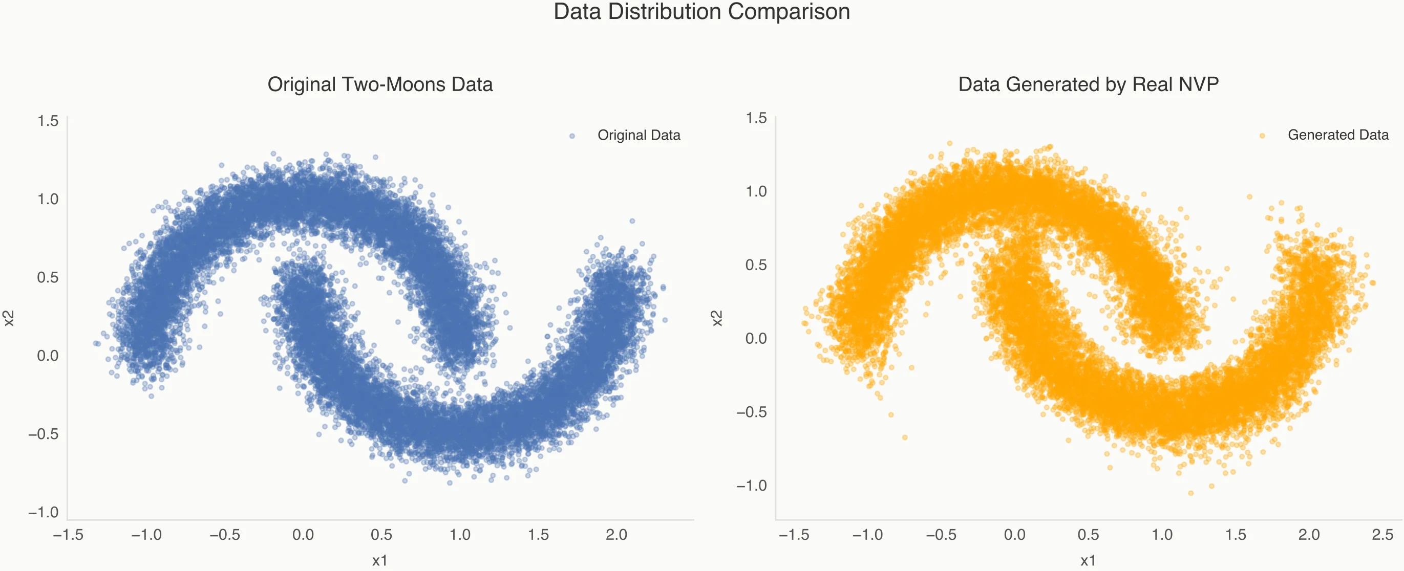
A flow trained on noisy two-moons data can concentrate probability around the crescents. Assessing that fit requires a specified noise level, preprocessing, architecture, optimizer, seed, and held-out likelihood. A visually plausible sample does not establish equality of distributions, and a likelihood number without those settings is not a reproducible result.

There is also a structural limit: a diffeomorphism of the full Euclidean space applied to a Gaussian retains positive density everywhere. It can approximate a gap with low density, but cannot produce an exact zero-density open gap or a distribution supported only on noiseless curves. Adding observation noise changes the target being modeled.

The tractable likelihood is the model’s density, evaluated through change of variables. Its agreement with data remains an empirical question.