Spectral Pollution in Kernel DMD: Why More Modes ≠ More Truth

This post is a continuation of:

Why Eigenvalues Lie: Pseudospectra for Non-Normal Operators

Claim: In kernel DMD and EDMD, many Koopman eigenvalues and modes are not properties of the underlying dynamical system. They are projection artifacts—spurious spectral features introduced by finite-dimensional approximation, regularization, and sampling. Adding more modes often increases spectral pollution, not insight.

What you’ll get:

The precise assumption that fails in “more modes = more truth”.
A concrete mechanism: Galerkin projection + high resolvent-norm regions produce fake point spectrum.
A minimal stability protocol to separate “mode you can trust” from “mode your basis invented”.

The Wrong Instinct

The standard Koopman workflow encourages exactly the wrong loop:

Increase dictionary size / kernel rank.
Compute more eigenvalues.
Treat denser spectra as “more structure”.

In non-normal, infinite-dimensional problems, that loop manufactures “structure” as fast as it reveals it.

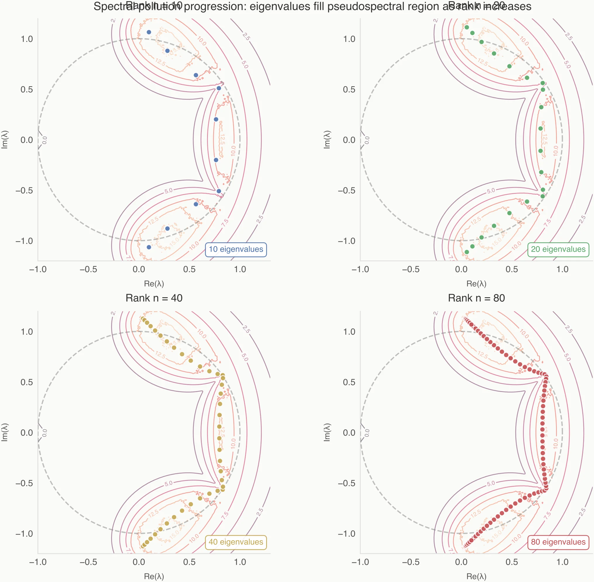
If you’ve seen eigenvalue plots that grow into a dense annulus as you increase rank (the “Ring of Fire”), this is the same phenomenon: you’re watching a finite model discretize sensitivity/continuum, not discovering a new family of physical modes.

One way to say this without folklore is: the ring often tracks level sets of the resolvent norm,

which a finite-dimensional projection turns into a contour of reported eigenvalues.

Resolvent geometry and spectral pollution — Figure 1 — Resolvent geometry (pseudospectrum). Background contours show level sets of the resolvent norm for a non-normal operator (proxy for a Koopman operator). The point is not “where eigenvalues are”, but where the operator is sensitive: large resolvent norms create regions where finite approximations tend to report spectrum. (The dotted points here are the true eigenvalues of ; the dashed circle is the unit circle.)

Finite projections do not “discover” spectrum; they discretize resolvent geometry.

Spectral pollution progression as rank increases — Figure 2 — Resolvent geometry → spurious eigenvalues (discretization). Overlaid points are eigenvalues of the compressed operators for increasing projection dimension . As grows, eigenvalues populate regions where the resolvent norm is large—even though these points are not eigenvalues of the underlying operator. Finite-rank projection discretizes sensitivity (pseudospectrum) into point spectrum, producing spurious Koopman modes.

The Hidden Assumption

When we compute Koopman spectra from data, we implicitly assume:

Finite-rank approximations preserve the spectral structure of the true operator.

That assumption is false in general. The Koopman operator acts on an infinite-dimensional function space. Kernel EDMD replaces it with a Galerkin projection onto a finite subspace. This is not a benign truncation; it fundamentally changes the spectral problem.

Even if the approximation converges in operator norm, its point spectrum need not converge to the true spectrum. New eigenvalues can appear that have no counterpart in the original operator. This phenomenon is called spectral pollution.

One subtlety worth stating explicitly: in practice, EDMD/kernel EDMD rarely achieves operator-norm convergence from finite data. The point here is stronger: even if it did, spectral convergence would still not follow.

The Mathematics of the Mirage

Let be the Koopman operator and be the projection onto your -dimensional dictionary. The object you actually diagonalize is the compressed operator:

In the limit you might expect spectral convergence, but operator theory does not give you that for free: convergence in the strong operator topology does not imply spectral convergence.

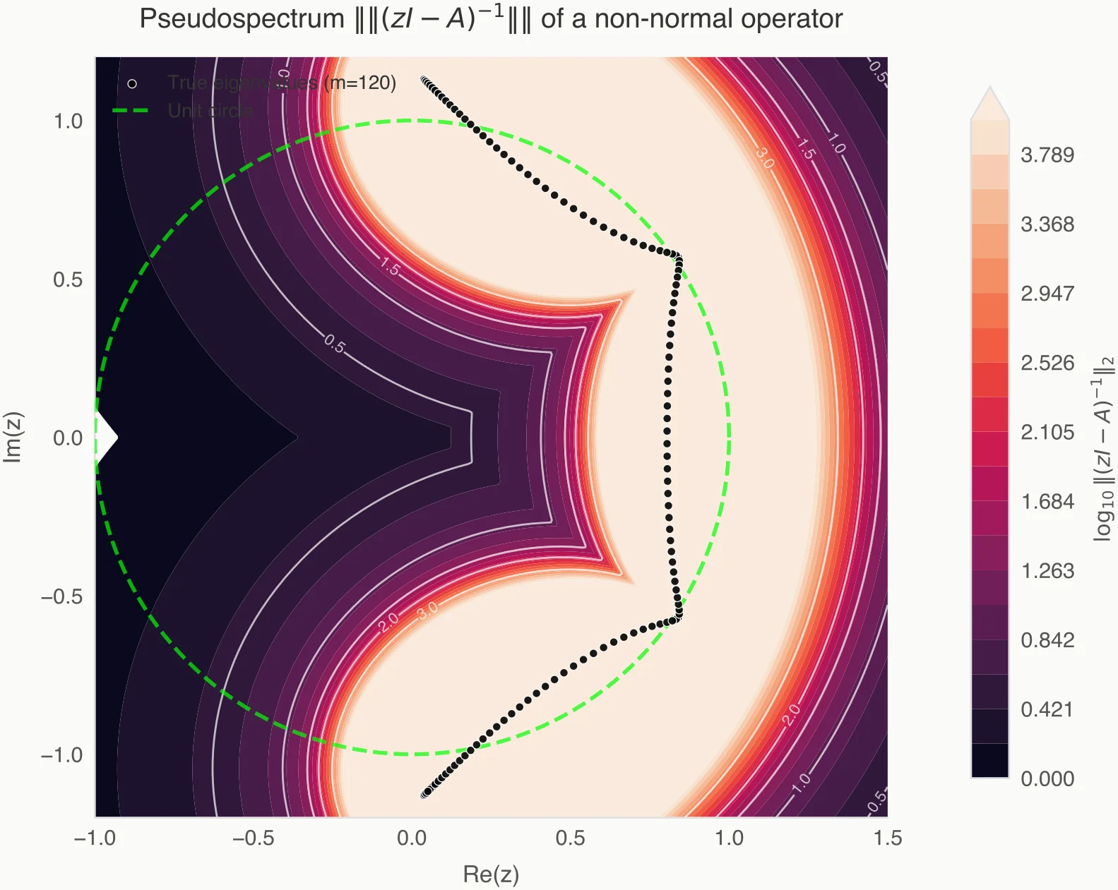
In non-normal settings, the spurious eigenvalues are often driven by the **-pseudospectrum**:

If your projection “touches” a region where the resolvent norm is high, the finite matrix will happily report an eigenvalue there, even if the true operator is invertible at that point. You are seeing sensitivity, not identity.

What Spectral Pollution Actually Is

Spectral pollution occurs when a finite-dimensional approximation produces eigenvalues that:

Do not converge to any true eigenvalue of the underlying operator.
Persist or move unpredictably as model capacity increases.
Appear inside gaps of the true (often continuous) spectrum.

In Koopman analysis, this is especially dangerous because the true operator often has a continuous spectrum, while the approximated operator always has a discrete spectrum. EDMD is forced to "invent" eigenvalues to fill the gap. These are not physical modes; they are numerical mirages.

This is not a numerical accident; it’s structural. A finite matrix can only give you point spectrum. Many mixing/chaotic systems generically do not—so the approximation has to discretize something (often a continuum) into “modes”.

A useful precision statement is:

In many mixing systems, the limiting lies in the continuous spectrum rather than the point spectrum. The finite model is not converging to an eigenvalue—it is discretizing a continuum of spectral sensitivity.

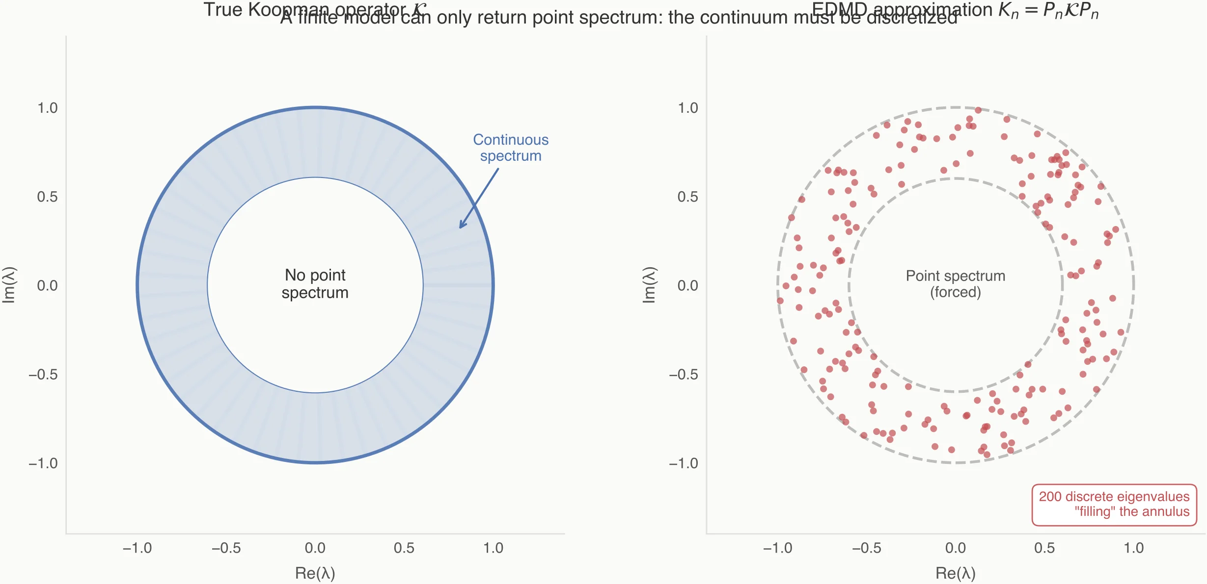
Figure 3 — Continuous spectrum vs finite matrix spectrum. Structural mismatch between infinite- and finite-dimensional spectra. (Left) The true Koopman operator may have predominantly continuous spectrum (shaded region). (Right) Any finite-dimensional approximation necessarily has only point spectrum. When EDMD or kernel DMD is applied to systems with continuous spectra (e.g. mixing or chaotic dynamics), the approximation must invent discrete eigenvalues to represent a continuum. These eigenvalues are not Koopman eigenvalues in the point-spectrum sense.

A finite matrix can only return eigenvalues, even when the true operator does not have them.

Why Kernel DMD is Especially Vulnerable

Implicit Dictionaries: The RKHS feature space is high-dimensional, but the effective rank is controlled by data and regularization. This obscures the true approximation dimension.
Non-Normality: Koopman operators are generically non-normal. Projection error is therefore amplified in the spectrum, not damped.
Sampling-Driven Subspaces: The Galerkin subspace is spanned by data-dependent features. Change the data slightly, and the spectrum changes.

Non-normality is not a vibe-word here; it changes what the resolvent means. For a normal operator, you have the clean identity

whereas for non-normal operators the resolvent norm can be large far away from the spectrum. Kernel DMD then tends to approximate regions of large resolvent norm and discretize them into eigenvalues.

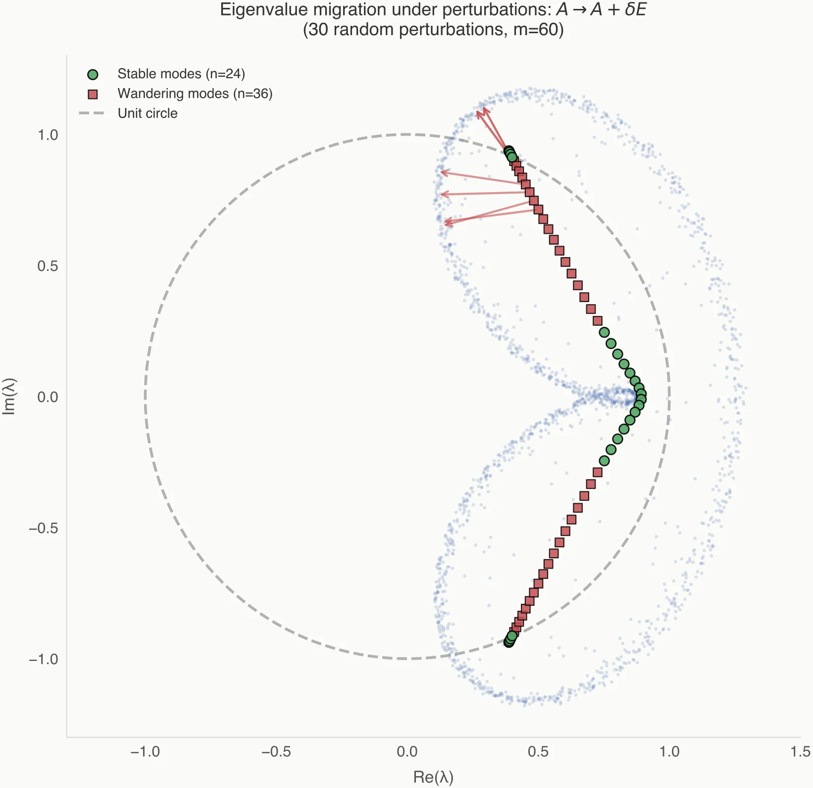
Figure 2 shows the practical consequence: as you increase rank, the reported eigenvalues “fill in” regions of high resolvent norm.

"More Modes" is Not a Neutral Choice

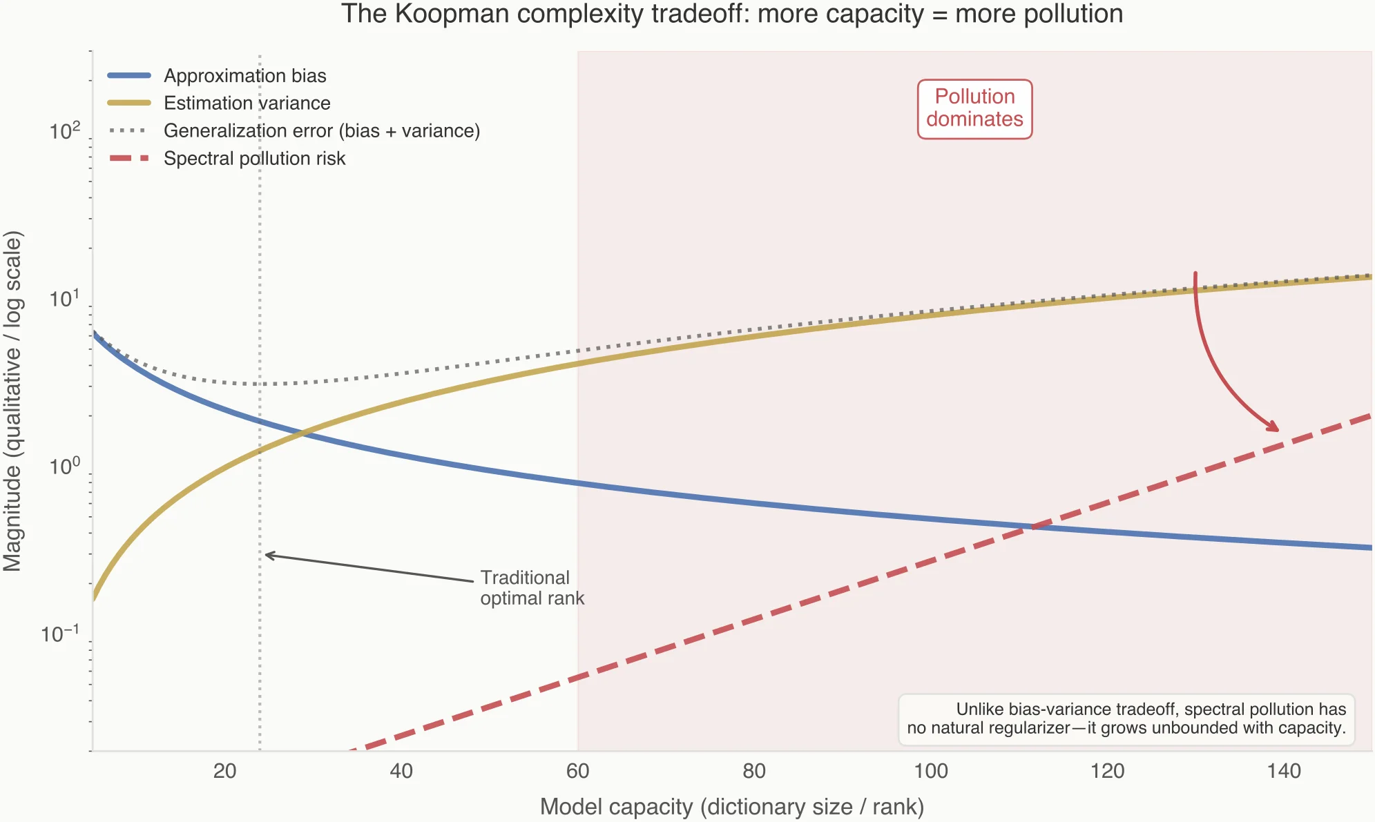
Increasing the rank of a Galerkin approximation does three things:

Reduces bias.
Increases variance.
Creates new spectral degrees of freedom with no physical anchor.

In systems with continuous spectra (chaotic or mixing dynamics), there is no discrete set of modes to converge to. The approximation must manufacture them. What you see as "emerging modes" are often projection-induced discretizations of a continuum, not discoveries. This is why eigenvalue plots often become busier but not more stable as model size grows.

Figure 5 — Bias–variance–spectral freedom tradeoff. Increasing rank is not a neutral operation. As dictionary size or kernel rank increases, approximation bias decreases and variance increases, but so does the number of unconstrained spectral degrees of freedom. In systems without isolated Koopman eigenvalues, additional modes often correspond to projection-induced discretizations rather than new dynamical structure.

The role of regularization in kernel EDMD is closely analogous to its role in kernel regression: both stabilize an ill-posed inverse problem in a high-dimensional RKHS. In regression, this has no interpretational cost—eigenvalues of the kernel matrix are not treated as physical objects. In Koopman analysis, however, we subsequently diagonalize the learned operator and interpret its spectrum. Regularization then stabilizes prediction while simultaneously reshaping eigenvalues, creating a gap between predictive success and spectral meaning.

A Minimal Stability Protocol (What to Actually Do)

If you take one thing from this post, take this: treat modes like hypotheses. Try to kill them.

Protocol: a mode is only “structural” if it survives small, principled changes in the projection.

Subsample sensitivity: refit on 80–90% of the trajectories / snapshots.
Regularization sensitivity: vary ridge/Tikhonov by a small factor (e.g., , ).
Kernel sensitivity (kernel EDMD): vary bandwidth / lengthscale slightly.
Dictionary sensitivity (explicit EDMD): swap a few basis functions or reduce degree by 1.

If an eigenvalue/mode migrates qualitatively under these changes, treat it as basis-dependent, not “the system”.

One practical diagnostic that often beats eyeballing eigenvalue plots: evaluate the one-step prediction error of the mode expansion under each perturbation. If the mode set changes but prediction error does not, you’re not learning new dynamics—you’re reparameterizing the same approximation.

Guardrail: stable prediction error does not certify that the modes are “true”. It only tells you the extra spectral detail is not buying predictive content, which is exactly when interpretation tends to go off the rails.

Formally: stability under projection perturbations is a necessary but not sufficient condition for a Koopman eigenpair to correspond to a genuine point-spectrum feature of . Instability falsifies interpretation; stability only licenses further scrutiny.

Figure 4 — Eigenvalue migration under small perturbations (stability test). Stability as a diagnostic for spectral meaning. Eigenvalues of a kernel EDMD approximation under small, principled perturbations of the projection (data subsampling, regularization strength, kernel bandwidth). Robust spectral features remain localized across perturbations, while projection-induced eigenvalues migrate substantially. Notably, these spectral changes often occur with negligible change in prediction error, indicating reparameterization rather than discovery of new dynamics. Spectral instability falsifies interpretation; stability is a minimum requirement, not a guarantee of correctness.

Practical Guidance

If you are using kernel DMD or EDMD, be skeptical when:

Adding modes changes qualitative conclusions.
Eigenvalues migrate under mild regularization changes.
Spectra densify without stabilizing (the "Ring of Fire" effect).

Internal Rule of Thumb: If a mode cannot survive a small change in the projection (e.g., subsampling the data or slightly shifting the kernel bandwidth), it does not describe the system—it describes your basis.

Conclusion: Projection Creates Structure

The most dangerous misconception in Koopman analysis is that all extracted structure reflects the dynamics. In reality, finite-rank projection is an active participant. It creates spectra, it doesn't just reveal them.

Spectral pollution is the default failure mode when infinite-dimensional dynamics are forced into finite representations. Understanding this shifts the focus from collecting more modes to identifying which spectral features are structurally real.

What this does not say:

Not all modes are fake; some systems do have robust, isolated spectral features.
Koopman/EDMD are not useless; they are useful when you treat spectra as hypotheses and test stability.
Stability is not completeness; it’s a minimum bar for interpretability.

Projection is not a passive lens—it is a generative mechanism.

More modes do not mean more truth. Stability does.

These effects are classical in numerical spectral theory for non-normal and indefinite operators; Koopman methods inherit them wholesale.