Eigenvalue Sensitivity: Pseudospectra for Non-Normal Operators

For a strongly non-normal matrix, a small perturbation can move eigenvalues much farther than its norm would suggest. Pseudospectra describe that sensitivity and help distinguish nominal stability from robustness to a specified amount of error.

In data-driven spectral methods—Dynamic Mode Decomposition (DMD), Koopman operators, kernel EDMD—we routinely do the same move: fit an operator from finite data, compute eigenvalues, and read off stability/decay/oscillation as if those points were intrinsic. That move has an implicit assumption:

• Eigenvalues are stable summaries of the operator.

For non-normal matrices, that assumption needs checking. Sampling, noise, and regularization affect the fitted matrix, and the map can be sensitive to their effects. Relating a finite matrix to an infinite-dimensional operator requires additional approximation arguments.

The relevant question is: given a bound on operator error, where could the spectrum move? A pseudospectrum answers this question for a chosen norm and error tolerance. It does not supply the error bound itself.

Related: Finite-dimensional projection creates an additional issue: spectral pollution. Its relationship to pseudospectra requires care:

• Spectral Pollution in Kernel DMD: What Projection Can Change

Normal vs. Non-Normal: Where Intuition Breaks

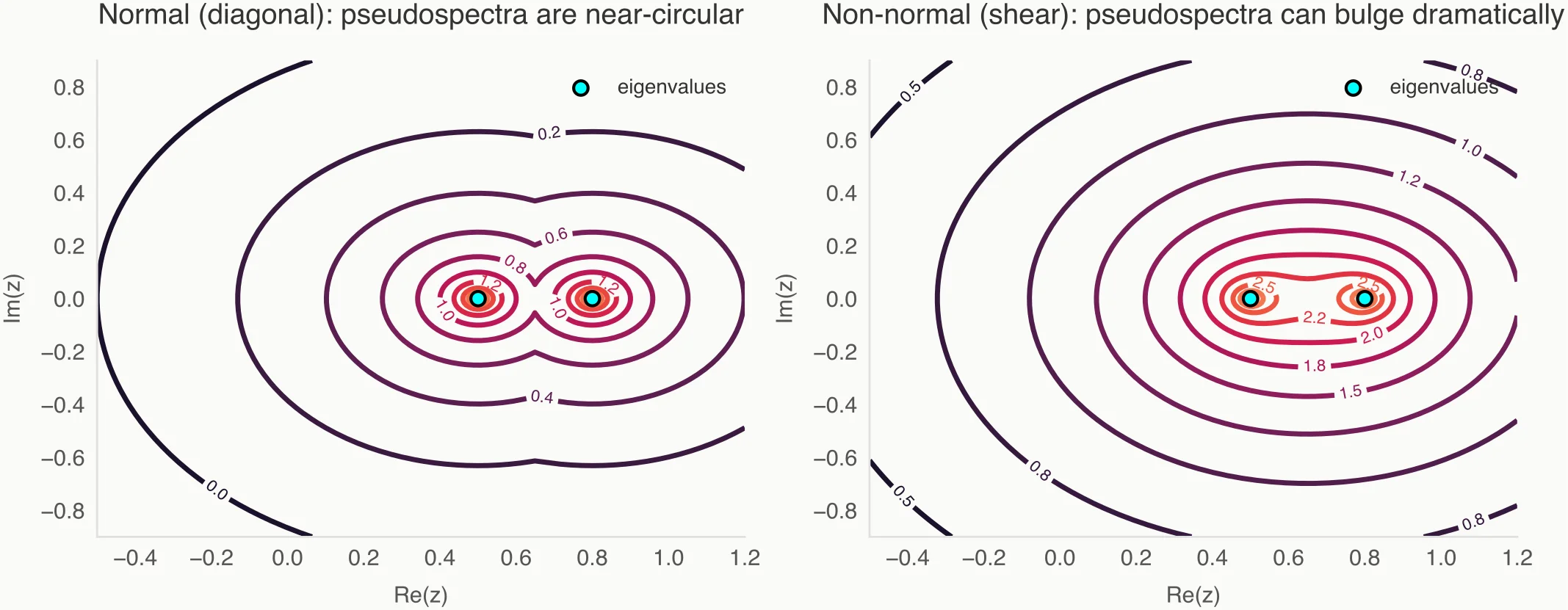
A normal matrix satisfies and has an orthonormal eigenbasis. Hermitian matrices are a special case. In the Euclidean operator norm, every eigenvalue of a perturbed normal matrix lies within the perturbation norm of its original spectrum.

Matrices describing shear and transient amplification can be non-normal even when all their eigenvalues indicate asymptotic decay.

Informally, an operator is non-normal if it does not commute with its adjoint:

A non-normal matrix has no orthonormal eigenbasis. If it is diagonalizable, its eigenvectors may be nearly linearly dependent; a defective matrix has no full eigenbasis at all. Non-normality permits sensitivity, but its magnitude must be quantified for the particular operator and norm.

This also depends on the function space: an invertible measure-preserving system has a unitary, hence normal, Koopman operator on the corresponding space. A fitted finite matrix need not inherit that property.

The Eigenvalue Instability Problem

Within a fixed finite-dimensional model, write the estimated matrix as:

where is a perturbation matrix representing noise or approximation error.

A concrete example is:

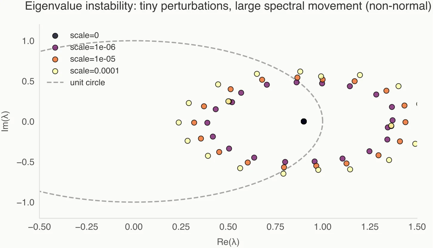
Both eigenvalues of are zero, but those of are , while . For , an error of size produces eigenvalues at . Sensitivity is a quantitative statement about this matrix, not a reason to discard all eigenvalues.

Enter the Pseudospectrum

For a finite matrix , use the closed -pseudospectrum in the Euclidean operator norm, with :

Equivalently, . These are exactly the eigenvalues attainable under complex perturbations of norm at most . The explicit union includes eigenvalues, where the inverse is undefined.

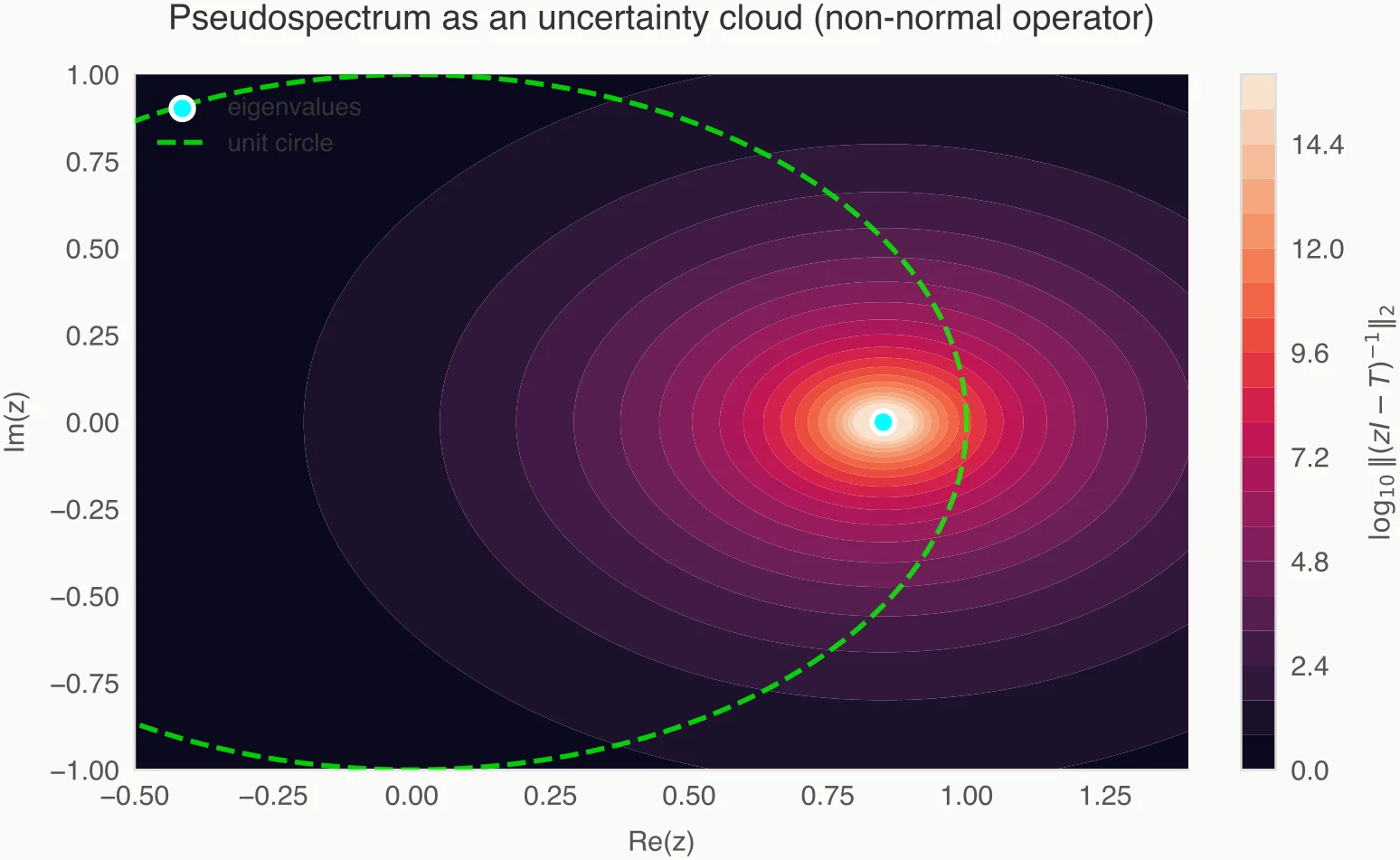
As increases, these sets form nested regions in the complex plane. Their boundaries are contours of the smallest singular value of .

If the matrix is normal, this set is the union of closed disks of radius around its eigenvalues. But for non-normal operators, these regions can expand dramatically, stretching far away from the eigenvalues, swallowing large portions of the complex plane.

For definitions and the perturbation interpretation, see Trefethen, Pseudospectra of Linear Operators.

Containment: What Pseudospectra Actually Guarantee

If and are matrices on the same space and , then:

This is an outer bound: a point in the pseudospectrum is a possible spectral location, not a confirmed eigenvalue of the unknown system. Tight regions constrain uncertainty; broad regions indicate sensitivity at the chosen tolerance.

Crossing the unit circle for a discrete-time model, or the imaginary axis for a continuous-time generator, indicates a possible destabilizing perturbation. It does not establish that the unperturbed system is unstable or predict the onset of turbulence.

Why This Matters for Data-Driven Operators

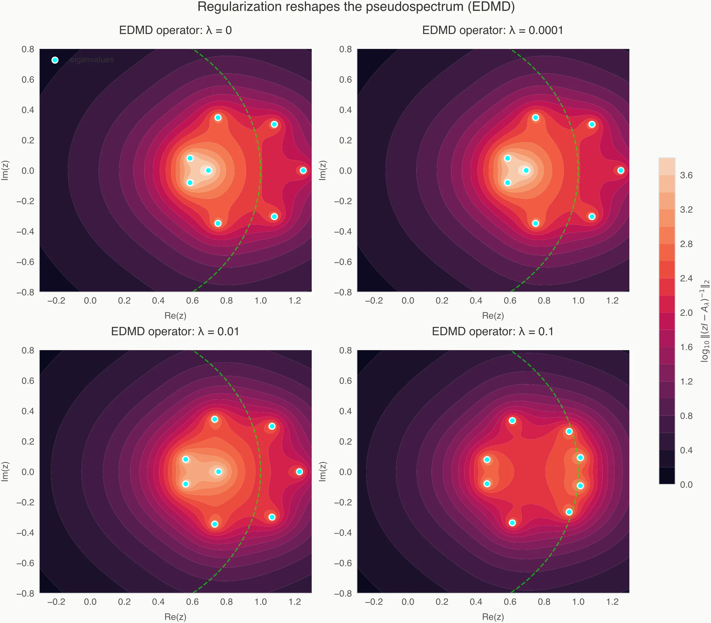
Finite-data estimation and regularization change a fitted EDMD matrix. Pseudospectra can describe its sensitivity to additional matrix perturbations, provided the norm and tolerance are specified.

Projection from an infinite-dimensional Koopman operator is a separate approximation step. A finite matrix and that operator act on different spaces; treating their difference as a small matrix requires an identification of the spaces and an error estimate. A pseudospectrum computed from the fitted matrix alone cannot supply either.

Likewise, changing regularization changes the fitted operator and potentially its pseudospectrum. The resulting regions do not automatically contain the spectrum of the full Koopman operator.

Pseudospectra vs. "Spectral Pollution"

Spectral pollution occurs when approximating spectra have limiting points outside the spectrum of the original operator. The resolvent of the projected matrix becomes singular at every one of its eigenvalues, including those introduced by projection. A large resolvent norm at a computed eigenvalue therefore cannot certify its physical meaning.

The missing quantity is error relative to the original operator. For a candidate observable , its normalized Koopman residual is:

This includes the component lost by projection. A small residual supports an approximate eigenpair at that tolerance, but can also reflect continuous spectrum or non-normal sensitivity; it does not alone prove an exact eigenfunction exists.

Residual Dynamic Mode Decomposition develops data-driven estimates of such residuals with error-control and convergence results under its assumptions. This supplies information beyond the resolvent of the compressed matrix.